It is the English
translation of article published in a
journal "Bulletеin assciaсii "Istorij i computer", Moscow, 1983, N 31. P. 266-269.
S. Nefedov
The elementary
model of agricultural population
The significant quantity of articles is
devoted to study of dynamics of the population in an agricultural society with
the help of mathematical models[1]. However
many models contain unknown coefficients, which influence their behavior. In
this brief note we offer the elementary differential model, which has no
uncertain parameters.
Let N(t) is a
population at the moment t. K(t) is stores of a grain after the collecting of
crop measured by an amount of minimum annual portions (1 portion is
approximately 240 kg of a grain). r
is a growth rate of the population in congenial conditions. A square of
sowings and a crop depend on a population. They aspire to some constant, when
the population grows. We shall consider,
that the crop is determined by the formula P=aN/(N+d),
where a and d are some constants. We use the usual logistics equation for
exposition of dynamics of the population
![]()
(1)
К is a current capacity in
this equation. This magnitude corresponds to an number K(t) of the accumulated annual portions in our case. N portions is spent for one year, and
the accretion of stores will be equal
![]()
(2)
So, we have the elementary system of two differential
equations (1) - (2). This system has a position of equilibrium, when the
population and the stores remain constants. It is a point K0= N0 = a-d.
If we fasten N
to 0 in the formula for dP/dN, we shall receive a/d – a crop (in an amount of portions),
received by one farmer in congenial conditions (when the population is small and he can cultivate a maximum
square). Thus, the magnitude q = a/d
shows, how much man (including itself) one farmer can feed in congenial
conditions (or how much families one peasant family can feed). It is known,
that q changes in limits 1.2 < q < 2 usually. It is convenient to express a and
d through q and N0:
d= N0/(q-1), a= qN0/(q-1).
N0 is known (or we can equate it to
1 conditionally). So in this model we have two constants r and q, having real
sense and varying in known limits: 0,01
< r < 0,02, 1,2 < q < 2.
The usual
methods of dynamic systems research allow to establish, that the system (1) -
(2) has characteristic numbers
![]()
( Magnitude D < 0 in all
range r and q). It means, that the system (1) - (2) generates damped
oscillations. First oscillations can have various period, but when curve comes
nearer to position of equilibrium, period is close to
![]()
The
period T increases, when r and q decrease, and period T decreases, when r and q
increase.
|
q\r |
0.01 |
0.02 |
|
1.2 |
154 |
110 |
|
2.0 |
89 |
63 |
Tab. 1. The period of oscillations at various
r and q (in years).
The first cycle can be much longer than the usual
extent of a cycle. The presence of the large stocks makes the illusion of well-being, but
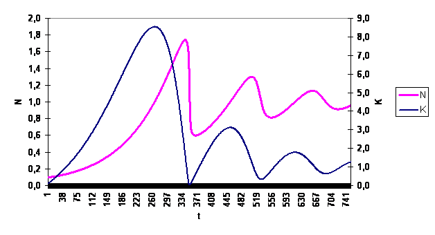
when the stocks are exhausted, the demographic catastrophe comes (fig. 1). The population can decrease in 2-4 times for
short time. The abundance of free
grounds occurs after the catastrophe, the population grows again, but the
excessive growth results in a catastrophe again. The second cycle is closer to
the standard period T, and the fall of a population has the smaller sizes. Oscillations gradually decrease in next cycles, and the
reduction of a population has no catastrophic character now.

Fig. 1 Example of account on model (r=0,016, p=1,2).
|
q\r |
0.01 |
0.02 |
|
1.2 |
0,46 |
0,33 |
|
2.0 |
0,64 |
0,53 |
Tab. 2. Factor of reduction of amplitude
for one cycle (for cycles near to a point of stabilization).
Thus, the dynamics of an agricultural population has
oscillatory character. Near to point of stabilization the period of oscillations has the extent of
one-two century, and the amplitude decreases approximately twice for one cycle.
The oscillations fade theoretically, but
in practice various casual influences remove the systems from a position of equilibrium, and a new series of fading oscillations
begins then. Such picture of fading oscillations was received earlier by J. Komlos and S. Nefedov at
modeling the growth of the population of Europe in 13th-18th
centuries[2].
The author thanks professor Peter Turchin for the
useful discussion of work.
References